Testing a Countercyclical Approach to Asset Allocation

And answering the question: "why not 100% equities?"

Note: This is part 3 of a series on asset allocation. To download our full 50-page report, please click on the link at the bottom of this email.

Reading this paper, investors might ask, per the telling title of Richard Thaler and Peter Williamson’s influential piece, “Why Not 100% Equities?” In lock-step with Warren Buffett and David Swensen, they argue that the best way to increase returns is to expand allocation to equities, with an all-equity portfolio at the extreme. While it is true that a simple buy-and-hold equity strategy could have potentially provided attractive returns to a patient investor over the past half century, that performance came with two significant drawbacks: painful drawdowns and significant stretches of time when the all-equity strategy produced low single-digit or zero returns.

We sought to design a strategy that would overcome these drawbacks. We believe a more strategic asset allocation model could pass three key tests:

Below we show the results of back-testing our strategy over a 50-year span since 1970. We also tested our asset allocation strategy against these stated goals. Following these test results, in the section entitled “Total Performance Contribution,” we give a detailed explanation of which aspects of the strategy we attribute to its performance in these tests. First, the results:

Test 1: Reducing Drawdowns

The first test is to produce a portfolio with drawdowns comparable to a 60/40 portfolio and significantly lower than an all-equity portfolio such as the S&P 500.

We believe this strategy would have been successful in avoiding the major drawdowns of the all-equity approach and producing drawdowns that are better or comparable to a 60/40 portfolio. The max drawdown on the portfolio over the full period was 15%, during the ’70s recession.

Figure 1: Historical Drawdown Comparison (1970–2020)

Source: Verdad. Note: Drawdowns calculated on a quarterly basis.

Test 2: Avoiding Lost Decades and Improving Consistency

The S&P 500 and 60/40 portfolios both resulted in long stretches of zero returns historically, a tough pill to swallow for investors. How did our strategy perform during the long bad stretches for stocks and bonds? Below we show returns by decade for our strategy, the all-equity portfolio, and the 60/40 portfolio. These returns are nominal, so we also show the inflation rate over the same period (as measured by the consumer price index, or CPI).  Green boxes highlight periods when the S&P 500 and the 60/40 portfolio experienced “lost decades.”

Figure 2: Comparative Total Period Returns (1970–2020)

Source: Verdad

In the two lost decades, the 1970s, when stagflation reared its ugly head, and the 2000s, when the market experienced two major recessions (in ’01 and ’08), this strategy produced double-digit nominal returns. This strategy produced consistent returns, decade by decade, based on our analysis.

The only time this strategy produced returns below the S&P 500 was during the great growth market of the 1990s, while performing at par with the S&P 500 in the 2010s. And even when it underperformed in the 1990s, our back-test showed that the returns were nearly 13%—not bad for an approach that is purposefully designed for consistency and drawdown reduction.

Test 3: Beating an All-Equity Portfolio

To counter Buffett’s argument that the best way to increase returns is to expand allocation to equities, with an all-equity portfolio at the extreme, we sought to produce a strategy that beats that benchmark. The chart below shows the comparative performance over the entire testing period for our strategy, an all-equity portfolio, and a 60/40 portfolio.

Figure 3: Comparative Performance (1970–2020)

Source: Verdad

We believe implementing our strategy since 1970 would have outperformed equities by about 500bps per year, all with a superior risk profile: a maximum drawdown of 15% and a Sharpe ratio of 0.8. We observed that the strategy’s risk metrics, in fact, were better than those of the 60/40 portfolio, despite this strong outperformance of the equity market.

From our perspective, our strategy would have significantly outperformed an all-equity or 60/40 portfolio in three of the past five decades, the bull markets in the 1990s and 2010s being the exceptions. In fact, in the past growth decade, our back-test shows that our strategy would have performed in line with a 60/40 strategy. We can see the strategy’s performance relative to benchmarks over time by charting the value of our countercyclical investing strategy divided by the value of its benchmarks, an all-equity and a 60/40 approach.

Figure 4: Countercyclical Investing Portfolio Value Divided by Benchmark Portfolio Value (1970–2020)

Source: Verdad

We believe the value over time of an investment in our proposed strategy could have been significantly higher than the value of an investment in the S&P 500 or a 60/40 portfolio. That said, there were two stretches of time when the S&P 500 and 60/40 portfolio delivered more value: the years ahead of the Dot-Com bubble and the years following the 2008 Financial Crisis. Both of these periods were defined by very high returns for the S&P 500. This helps illustrate one aspect of this asset allocation model: during periods when the S&P 500 is returning more than 15% per year, we noticed that the strategy tends to underperform a 100% equity portfolio. Conversely, when the S&P 500 is returning less than 15% per year, the strategy tends to outperform. This is to say that the benefits of this approach are truly realized not in good times, when the market rewards all investor behavior, but rather in bad times, when those who are unprepared stand to suffer greatly and those who are prepared stand to reap large rewards. In the chart below we show annualized five-year rolling real returns for the S&P 500 on the x-axis and our strategy’s annualized five-year rolling excess returns versus the S&P 500 on the y-axis.
 

Figure 5: 5-Year Rolling Strategy Excess Returns over S&P 500 vs. S&P 500 Real Returns

Source: Verdad

This makes sense for a strategy that has about an 88% upside capture ratio versus the S&P 500 but has only a 21% downside capture, as shown in the graph below. The upside and downside capture ratios indicate the degree to which our strategy outperforms a broad market benchmark during periods of market strength and weakness. We calculate the upside capture ratio by taking the strategy’s returns during quarters when the benchmark had a positive return and dividing those returns by the benchmark returns during those periods. Conversely, we calculate the downside ratio by taking the strategy’s returns during quarters when the benchmark had a negative return and dividing the strategy’s returns by the benchmark returns during those periods.
 

Figure 6: Countercyclical Investing Strategy Capture of Benchmark Upside and Downside (1970–2020)

Source: Verdad

This very limited downside capture is a key distinguishing attribute of our strategy. Over longer periods, we believe the countercyclical investing strategy wins by not losing and retaining gains despite market turbulence. The chart below shows that the strategy outperformed over 85% of 10-year periods, 72% of five-year periods, 67% of three-year periods, and 55% of one-year periods, based on our analysis. Conversely, the strategy is most likely to underperform during prolonged bull markets with low volatility. When the strategy underperformed, it was almost all during periods of >15% returns on the S&P 500.
 

Figure 7: Comparative Analysis of Average Annualized Rolling-Period Returns (1970–2020)

Source: Verdad

Total Performance Contribution

Of the countercyclical investing strategy’s three key tactics (i.e., countercyclical investing using business cycle indicators, dynamic asset allocation in response to changing economic environments, and trend-following to protect against short-term economic shocks), we wanted to understand better which tactic contributes most to the strategy’s success, so we looked at the data from three different angles.

First, we checked if our defined portfolios perform as expected in their namesake economic states as predicted by the cycle indicators. Below we show portfolio and asset-level performance by economic environment.

Figure 8: Portfolio and Asset Performance by Economic Environment (1970–2020)

Source: Verdad
 

We confirmed that our defined portfolios could have been top performers during their namesake economic states as predicted by the cycle variables. Note that we apply trend-following to the S&P 500 and gold in inflation and growth portfolios to enhance returns and reduce drawdowns, as shown in Chapter 2, Figures 10 and 13 of the full paper.

Second, we looked at how portfolio switches versus a buy-and-hold approach in an all-equity or a 60/40 portfolio would have performed. Specifically, we looked at three-, six-, and 12-month forward returns from the moment a portfolio switch is triggered by a shift in the high-yield spread and/or the slope of the yield curve.
 

Figure 9: Forward Returns When a Portfolio Switch is Triggered

Source: Verdad

We found that our ability to predict changing economic environments contributed to our excess returns over the all-equity and 60/40 portfolio strategies consistently over three-, six-, and 12-month periods. We looked to see if these signals degraded in predictive power over time as measured by changes in relative forward returns over time, but we found no general trend suggesting that the predictive power might be diminishing.

Finally, we completed a performance attribution analysis to isolate each elements’ magnitude of contribution to the overall performance of the strategy compared to a 60/40 portfolio.

Figure 10: Performance Contribution Breakdown vs. 60/40 Portfolio

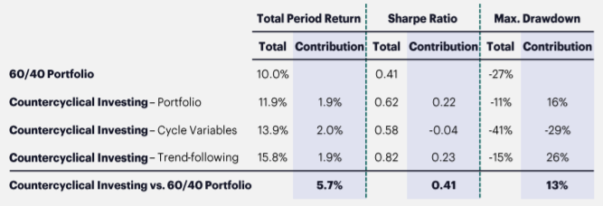
Source: Verdad

Overall, we found that the combined strategy could have contributed 570bps in excess of the 60/40 portfolio returns (and 500bps in excess of the all-equity portfolio returns). We found that each of our three pillars could have potentially contributed to the excess returns in a balanced way.