Designing a Countercyclical Strategy
How to Integrate Business Cycle and Trend Analysis
Note: This is part 2 of a series on asset allocation. To download our full 50-page report, please click on the link at the bottom of this email.
The four quadrants highlight two simple yet important facts: Our economy is dynamic, with no two decades remotely the same, and asset performance is driven by growth and inflation. We have seen that investors should overweight equities in growth environments and commodities in inflationary environments. In times when both growth and inflation are falling, high-quality fixed income has tended to provide the most reliable returns.
Generating alpha based on these insights requires two considerations. On the one hand, anticipating the direction of growth and inflation to allocate the portfolio to top-performing assets in each environment. On the other hand, avoiding major drawdowns to ensure capital is available to take advantage of the economic dislocations that provide the greatest profit opportunities.
Harvard’s Andrei Shleifer, along with some of the top researchers in behavioral finance, has developed a new model of investor psychology called diagnostic expectations. Their theory, grounded in substantial empirical work in markets, shows that investors extrapolate from the recent past in forming their return forecasts for the future and that they act on these backward-looking forecasts. This leads to short-term trends, with good news leading to expectations of more good news, leading to rising prices, or bad news leading to expectations of more bad news, leading to falling prices.
But this mental model is not only irrational, it is negatively correlated with rational models (a rational model, for example, would predict higher returns when prices are low and lower returns when prices are high). The big revelation of Shleifer’s paper is that these correlations represent a systematic and recurring error: “In particular, they are consistent with the presence of excessive optimism in good times and excessive pessimism in bad times: future realized earnings growth systematically falls short of expectations when past earnings are high and exceeds expectations when past earnings are low.” This explains why markets trend in the short term, yet they tend to mean revert in the long term.
We believe this theory provides an informative model for making decisions about asset allocation. During market panics—as we showed in Crisis Investing—investment returns are predictably higher. During crises, investors and lenders panic, selling assets at fire-sale prices due to an irrational extrapolation of recent bad economic news. We argue that investors should act counter-cyclically, loading up on riskier assets, especially small value stocks and higher-yielding bonds, during these windows. Conversely, when economic times are good, investors tend to neglect future risks and respond to reduced market risk premia by “reaching for yield” or piling into asset bubbles. During these times, we believe investors should take proactive steps to guard their portfolios from reversals in economic growth and from sudden spikes in inflation, incorporating recent price trends to make fast updates to their portfolios as new risks emerge. In short, we believe investors should follow Warren Buffett’s admonition, “Be fearful when others are greedy and greedy when others are fearful.”
In this section, we marry this behavioral finance model with the four-quadrant framework to propose a novel approach to asset allocation. This approach has three defining features:

Counter-Cyclical Investing Through Business Cycle Indicators
In a famous 1992 paper entitled “Common Risk Factors in the Returns on Stocks and Bonds,” Eugene Fama and Ken French expand their factor analysis of the US equity market to the bond market. They find that two factors - the slope of the yield curve and the spread between the yield on corporate bonds and government bonds - explain returns in both the bond and the stock markets. We rely on these two well-established business cycle indicators to drive our asset allocation decisions.
High-Yield Spread
We use high-yield credit spreads as our primary business cycle indicator, a metric on which we based our Crisis Investing research and which we have written substantially about in prior years. The spread measures the difference between the borrowing rate for below-investment-grade bonds and the corresponding US treasury spot rate. It is a contemporaneous indicator of investor sentiment about economic growth. We use this as our primary indicator because, as we have seen in Chapter 1, asset performance in growth environments in quadrant 1 (rising growth, falling inflation) and quadrant 2 (rising growth, rising inflation) tends to be less sensitive to inflation.
When the high-yield spread is wide, likely in a recession, it reflects the perceived risk of investing in below-investment-grade issuers, typically small and cyclical businesses, in bad times, hence the heightened risk premia. Paradoxically, this is an ideal time to load up on risky assets, specifically small value stocks, and to generally overweight equities, as these periods are often followed by recoveries and therefore high growth.
Below we show three-month forward change in real GDP growth and the three-month forward returns for small value stocks and the S&P 500 when high-yield spreads are above versus below the trailing 10-year median, which we use as a proxy for a business cycle length. Wider spreads are conducive to significant excess returns for small value stocks, while to a lesser extent benefitting the broader equities market. This is in line with our findings in quadrant 1 (rising growth, falling inflation) and quadrant 2 (rising growth, rising inflation).
Figure 1: 3M Forward Growth Rate Change and Asset Returns by High-Yield Spread (1970–2020)

Source: Verdad
Slope of the Yield Curve
When the high-yield spread is tight, suggesting slowing or negative growth, we incorporate an additional business cycle indicator: the slope of the yield curve. We use the yield curve to estimate the direction of inflation and differentiate between two falling growth environments: when inflation is rising in quadrant 3 (falling growth, rising inflation) and investing in real assets has delivered the best historical returns, and when inflation is falling in quadrant 4 (falling growth, falling inflation) and fixed income has worked better. The slope of the yield curve measures the spread between long-term and short-term government bonds (e.g., 10-year versus one-year) and has historically been a powerful indicator of business cycle stages: steep at business cycle troughs and flat at business cycle peaks.
Figure 2 on the following page shows the three-month forward average change in inflation and the three-month forward average returns for gold and Dow Jones investment-grade bonds in periods when high-yield spreads are tight. We have divided this economic condition into two subsets: when the slope of the yield curve is above versus below the trailing 10-year median, which we use as a proxy for a business cycle length.
When the high-yield spread is tight, flat slopes seem to be anticipating rising inflation and are conducive to excess returns in commodities and gold, while steep slopes seem to predict falling inflation and are conducive to excess returns in fixed income. This is in line with our findings in quadrant 3 (falling growth, rising inflation) and quadrant 4 (falling growth, falling inflation).
Figure 2: 3M Forward Inflation Change and Asset Returns by Slope of Yield Curve (1970–2020)

Source: Verdad
Risk Reduction Through Trend Signals
As Shleifer noted, markets tend to trend in the short term as investors extrapolate from recent news. This leads to investor overreaction to both good and bad news and contributes to the excess volatility of markets. We believe investors should incorporate these short-term price trends into their asset allocation decisions to mitigate downside risk and enhance returns.
Volatility tends to cluster and using simple trend-following rules can help investors reduce their portfolio volatility, giving them more capital to make counter-cyclical investments. Trend following can help hedge against both sudden negative shocks to growth and sudden positive shocks to inflation. This strategy, also known as time series momentum, works across many different asset classes and geographies and is one of the most robust factors in the academic finance literature.
In this paper we use a simple definition of trend: whether current market prices are above or below the 200-day moving average. Specifically, when the price level of the risky asset (e.g., S&P 500 or gold) falls below its 200-day simple moving average for five consecutive days, we reallocate the risky share of the portfolio to 10Y US treasuries.
Moving average rules are the most basic form of trend following, and we are aware of research suggesting ways to improve on simple moving average rules. However, we use them here precisely for their simplicity, to avoid data mining.
Trend-Following Equities
The recent price movements in the S&P 500 have historically predicted short-term returns in the S&P 500 as well as the short-term trajectory of real GDP growth. Below, we show the average three-month forward S&P 500 returns and US real GDP growth rate from the moment the S&P 500 is above versus below its 200-day moving average.
Figure 3: 3M Forward Returns and Real GDP Growth by S&P 500 Value vs. 200-Day Moving Average (1970–2020)

Source: Verdad
This simple 200-day moving average rule can help investors shift between owning equities, the best performing asset class in growth environments, and owning government bonds, the best performing “no growth” asset. This rule is effective because the stock market’s price movements have real informational content about the trajectory of future growth, as academic research has shown.
These results are still robust when we vary the time period of the moving average. We found similar results using a 60-, 120-, 200-, and 250-day moving average. Although the 120-day moving average rule had the best performance, we relied on the 200-day moving average because it is the most commonly used in the literature and by practitioners.
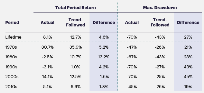
Below we show the annualized returns and maximum drawdowns for the S&P 500 total return index with and without trend following. We break down the results by decade.
Figure 4: S&P 500 Performance by Strategy and Decade (1970–2020)

Source: Verdad
We found that trend following is most effective at significantly reducing drawdowns. To quote Wes Gray of Alpha Architect, trend following is effective in protecting portfolios from “the most extreme loss situations.” Trend following has helped equity investors avoid drawdowns in all major recessions in recent history, as shown below.
Figure 5: Maximum Drawdowns by Strategy for S&P 500 Total Return Index

Source: Verdad
Trend-Following Gold
Similarly, the recent changes in the price of gold can be a powerful predictor of the short-term performance both of gold itself and of US inflation. Below we show the average three-month forward gold returns and inflation rate from the moment the gold price is above versus below its 200-day moving average.
Figure 6: 3M Forward Returns and Inflation Rate by Gold Price Level vs. 200-Day Moving Average (1970–2020)

Source: Verdad
The current price of gold relative to the 200-day moving average can help investors shift between owning gold, a reliable performer in inflationary environments in quadrant 2 (rising growth, rising inflation) and quadrant 3 (falling growth, rising inflation), and owning 10-year US treasuries, a reliable performer in deflationary environments in quadrant 1 (rising growth, falling inflation) and quadrant 4 (falling growth, falling inflation). As with the S&P 500, these results are robust to different moving average time windows.
Below we show the annualized returns and maximum drawdowns for gold prices with and without trend following. We break down the results by decade. Trend following reduces max drawdowns by about half.
Figure 7: Gold Performance by Strategy and Decade (1970¬2020)
Source: Verdad
By significantly reducing drawdowns, trend following can enhance long-term portfolio-level returns in a cost-effective way.
Our results confirm one of the most robust and well-studied phenomena of global financial markets: the power of trends. Along with Shleifer, other leading researchers such as Jeremy Siegel (Stocks for the Long Run) and Tobias Moskovitz, Yao Hua Ooi, and Lasse Pedersen (“Time Series Momentum,” 2012), point out investor overreaction to selloffs and underreaction in uptrends as likely reasons for short-term trend persistence. Moreover, Moskovitz et al. confirmed this persistence goes beyond global equities markets: it holds across commodities, bonds, and currencies too. AQR’s Brian Hurst, working with Ooi and Pedersen, looked at a century of evidence across multiple asset classes and found similarly favorable results. “Trends are pervasive features of financial markets,” they wrote.
Investors can use these trend signals to proactively harness the power of assets that respond positively and negatively to growth and inflation, avoiding major losses and reducing overall portfolio volatility. Incorporating these short-term insights over the long term helps significantly moderate drawdowns, preserving capital to make counter-cyclical investments in times of crisis.
Portfolio Allocation in Response to Changing Economic Environments
The four-quadrant framework is useful in understanding historic economic shifts and the drivers of asset performance, but it can be unnecessarily complex to implement in practice. Specifically, equities, the top-performing assets in growth quadrant 1 (rising growth, falling inflation) and quadrant 2 (rising growth, rising inflation), bear little sensitivity to inflation, as shown in Exhibit 1. So we simplified the framework to have only one growth portfolio for both rising growth environments, quadrants 1 and 2. We then constructed an inflation portfolio that is well positioned to profit from inflationary pressures and a slowdown portfolio designed to preserve capital when the economy is slowing.
Figure 8: Asset Allocation by Economic Environment

Source: Verdad, Bridgewater, Hedgeye
Our proposed portfolios are aimed at generating attractive returns in their namesake economic environments, as predicted by business cycle indicators.

This counter-cyclical asset allocation strategy combines the ability to estimate future economic environments through business cycle indicators, dynamic portfolio allocation in response to changing economic environments, and trend signals that provide a downside protection mechanism during economic shocks.
Figure 9: US Counter-Cyclical Investing Framework

Source: Verdad
We employ trend-following rules to the S&P 500 and to gold in the growth and inflation portfolios. Specifically, when the price level of the S&P 500 falls below its 200-day simple moving average for five consecutive days, we sell the S&P 500 and buy 10-year US treasuries. Conversely, we sell the 10-year US treasuries and buy the S&P 500 when the price level of the S&P 500 rises above its 200-day simple moving average for five consecutive days. Trend-following is applied to gold in the same way. When the price level of gold falls below its 200-day simple moving average for five consecutive days, we sell gold and buy 10-year US treasuries, and vice versa.
As a result of applying trend-following rules to the S&P 500 and gold, we held on average, a portfolio that looked like the below Figure 10.
Figure 10: Average Historical Portfolio Allocation (1970–2020)

Next week, we will explore the results of this strategy.