We Measure What We Can
Charlie Munger and Nassim Taleb have criticized volatility as a measure of risk. Are they right?
By: Verdad Research
There is a common idea in academic finance that is conspicuously dismissed by both contrarian investors and the popular culture: the claim that historical volatility is a good indicator of future risk. This idea is treated with derision in acclaimed films like Margin Call and The Big Short—and is a frequent source of controversy in MBA classes and undergraduate finance curricula.
“Using volatility as a measure of risk is nuts,” said Charlie Munger, in a refrain echoed in MBA classrooms across the country. “Risk to us is 1) the risk of permanent loss of capital, or 2) the risk of inadequate return.”
Munger is not the only investor who thinks this way. In 2007, Nassim Taleb’s book The Black Swan cast doubt on the entire exercise of using historical data to predict risk. To Taleb, the risk that matters is what remains after accounting for what can be calculated—true risk is the turkey’s first Thanksgiving, the short squeeze in GameStop, the grim reminder that induction is not proof. True risk cannot be measured – only respected.
But we believe that, despite these impassioned critiques, volatility as a measure of risk has three considerable points in its favor:
Volatility correlates strongly with the risks investors intuitively care about, such as drawdowns and defaults.
Volatility can typically be estimated from historical data much more accurately than most other proposed risk metrics.
Volatility correlates with itself across time, in both the short term (within a given asset class) and the long term (across asset classes).
At the risk of provoking the ire of a certain Lebanese weightlifter, we’d argue that volatility measures can significantly improve long-term investment decision making.
Let’s consider each of the key arguments in favor of academic volatility measures.
1. Volatility is correlated with the risks investors intuitively care about
First, we believe volatility is a reliable correlate of the risks investors seem to care about. Munger says that what matters to him is loss of capital, but more volatile assets have historically had much larger drawdowns. Compare the following two tables showing annualized return volatility and maximum drawdowns for major asset classes across two time periods: 1990 to 2005, and 2005 to the present.
Figure 1: Return Volatility, Max Drawdowns of Major Asset Classes, 1990–2023
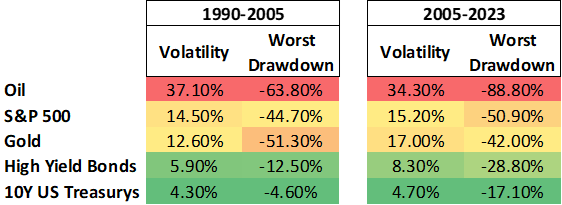
Source: Bloomberg Data
Across both time periods, volatility and drawdowns are highly correlated across asset classes, and volatility within the first period is a good predictor of volatility within the next period.
We see a similar pattern with default rates in corporate credit, where riskier bonds have exhibited both greater return volatility and higher default rates from 1988 to 2022. If you’re most worried about loss of capital, we believe volatility has been a good predictor of true loss of capital in credit.
Figure 2: Annualized Avg Returns, Default Rates, and Return Volatility by Credit Rating, 1988–2022

Source: Moody’s, Capital IQ
Now it is true that the relationship between volatility and drawdowns or defaults is not perfect. For example, 10-year Treasurys had consistent volatilities over the two periods shown above, but in the past two years they have realized their worst drawdown in over three decades—over 17%. Nothing like this occurred in the period from 1990 to 2005, and neither past drawdowns nor past volatility would have been helpful in predicting this. But this is not an indictment of volatility. It is an acknowledgement of the irreducible randomness of the path a portfolio may take.
2. Volatility can be precisely estimated using historical data
To better understand the precision of volatility and drawdown estimators, we will make use of a Monte Carlo approach: a simulation aimed at studying the behavior of a random system. As an experiment, we define a probability distribution of weekly returns that is designed to mimic the return distribution of a levered equity portfolio, fat tails and negative skewness included.
This is a highly simplified problem. True-to-life return distributions are not static, and the distribution we used, though not a normal bell curve, is still more “well behaved” than many real-world return distributions in our opinion. But even under these idealized conditions, we will see substantial difficulties in estimating risk via drawdowns.
The true annualized Sharpe ratio of this return-generating process, by construction, is 0.71. To understand the robustness of return, volatility, and drawdown estimators, we simulated 10 years of weekly data 10,000 times and analyzed the results.
Figure 3: 10 Years of Simulated Data, 10,000 Trials, Risk Metrics and Ratios

Source: Verdad Analysis
Tracking this strategy for a decade, we would obtain a highly precise estimate of its volatility, but we would still be left with a noisy estimate of its average return and a large interquartile spread in the realized drawdowns. The exact same investment strategy, in the exact same market environment, measured over a decade, could easily have maximum drawdowns that vary by over 15 percentage points. This variation is entirely due to chance.
In addition to the large spread in our sample maximum drawdown, there are other more subtle issues. Maximum drawdown necessarily increases with sample length. The longer the historical sample one considers for a given strategy, the more time there is for the biggest drawdown to be particularly large. But this says nothing about the strategy’s risk. Even worse, realized drawdowns for a given strategy tend to be correlated with the sample mean. If one was unlucky with drawdowns, average returns were probably also unfavorable. This becomes a problem when one attempts to weigh an estimate of risk against an estimate of return. Errors in estimation compound.
Investors might care about drawdowns, but drawdowns might not be a good indicator of the risks an investor took: they vary too much for no reason at all except for randomness. But volatility as a metric is highly precise. Realized historical volatility is often a decent proxy for the true volatility one should have expected in advance. This is why, despite its obvious limitations, mean-variance thinking has persisted in finance throughout the 21st century: what it attempts to capture, it captures well.
Why can volatility be estimated so accurately? In 1980, Nobel Prize winner Robert Merton wrote a seminal paper, entitled On Estimating the Expected Return on the Market, in which he argued that volatility estimates become more precise if one examines higher frequency data, while mean estimates do not. One can get “more volatility” to measure by sampling returns more frequently, increasing the effective sample size.
Perhaps our readers are convinced that drawdowns are a bad risk metric but still believe that only losses ought to be considered risk (a point that we’ve entertained in the past). Semivolatility is a metric that only includes the volatility of returns that are below some threshold, typically zero. The problem is accounting for the losses one doesn’t see when a strategy swings big and happens to win by sheer luck, particularly in a backtest. Strategies in development that make bold bets and lose get discarded; funds that do the same tend to leave the industry. If a strategy has the potential to make windfall profits, one should expect that it can either experience large losses or that it tends to lose money on average. This is not an iron law, but it is certainly much easier to construct a strategy that can experience large swings in either direction than one that only swings upward. Therefore, we believe realized volatility to the upside is usually evidence of the potential for realized volatility to the downside.
3. We believe volatility is systematically predictable
So now we know that volatility correlates with loss-of-capital metrics and that, unlike loss-of-capital metrics such as drawdowns, it can be estimated in a robust manner. This brings us to our final claim about volatility: that it is systematically predictable.
In 2003, Robert Engle won the Nobel Prize in Economics for a simple observation: return volatility tends to be autocorrelated and to cluster in time, which means that statistical models can make use of trailing realized volatility to predict future volatility.
There are many reasons why we believe this is true. First, when an extreme event occurs in the world, expectations among investors often diverge, which leads to trading and volatility as the market digests the news and equilibrates. But this process is not instantaneous. So if one witnesses a bout of volatility in the markets, it is reasonably likely that the bout is not yet finished. Volatility takes time to play out.
Second, asset returns depend on how investors respond to past returns. For instance, if an investor suffers a massive drawdown, he might receive a margin call and be forced to liquidate his positions. In this way, financial volatility often begets further volatility.
Finally, extreme events in the real world are themselves autocorrelated. A political upheaval is more likely if there has been a war or a famine. Earthquakes can cause blackouts, which can in turn reduce economic output. The world is fragile and interconnected.
To help visualize this relationship, we constructed a scatter plot of the one-month realized volatility of the S&P 500, measured against the previous month’s realized volatility, from 1988 to 2022. One can see that the relationship between past and future volatility has persisted over decades.
Figure 4: SPX 1M Realized Volatility vs Trailing 1M Realized Volatility, 1988–2022

Source: Bloomberg Data
Where do we go from here? Next week, we will make the case that volatility forecasting can be used to improve portfolio outcomes. But for now, we want to point out that Taleb and Munger aren’t necessarily wrong. There is nothing incorrect about having a utility function that prioritizes drawdowns over volatility. It just means that the utility Munger gets from a given investment strategy will depend more on randomness that ultimately cannot be controlled, beyond the control that a model of volatility (and autocorrelation in returns) permits. And Taleb is right about the importance of black swans. Volatility is a useful metric, but if it is used in an unsophisticated way, it can do more harm than good. We will present a framework for thinking about so-called “higher order risks” in the future.
Despite its limitations, we believe that volatility is one of the best risk metrics an investor can use, both as a measure of past risk-adjusted performance and as a forward-looking tool for navigating the future.