On Oil

Supply, Demand, and Mean Reversion in Oil Prices

The eighteenth-century economist Thomas Malthus became famous for his predictions that population growth would outpace agricultural production and cause a plunge in living standards to subsistence-level conditions. Malthus was right about population growth but wrong about agriculture: human innovation led to surging crop yields and a sharp drop in hunger despite world population rising into the billions, a story well documented in Nobel Prize­–winning cliometrician Robert Fogel’s The Escape from Hunger and Premature Death.
 
Two centuries after Malthus published his ideas, Stanford professor Paul Ehrlich updated Malthus’s thesis for the twentieth century, publishing The Population Bomb, in which he predicted that overpopulation would give rise to worldwide famine and severe resource scarcity in the coming decades. Heavily promoted by environmentalists, the book became a bestseller. But the economist Julian Simon figured Ehrlich’s predictions would be about as accurate as Malthus’s, and he convinced Ehrlich to agree to a $10,000 wager that the inflation-adjusted prices of any five commodities of Ehrlich’s choosing would be lower a decade hence.
 
A decade later, all five commodities were cheaper in real terms, just as Simon predicted. What Ehrlich missed was that the supply of natural resources is capable of overwhelming expansion, as technological breakthroughs can lead to drastic improvements in efficiency and productivity.
 
While oil was not part of the wager, the bet played out in a similar fashion for oil prices. We can see in the below chart that stagnant oil prices have led to equity underperformance for energy stocks over the last 40 years, with increased volatility from the big price swings in the oil market.
 
Figure 1: Buy-and-Hold Performance Indicators for Energy Stocks and Oil Futures (1983–2020)

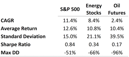
Source: Bloomberg, Verdad, Ken French Data Library

Over the long term, buying and holding oil futures and energy stocks have generated poor results relative to alternatives, particularly on a risk-adjusted basis. New sources of supply were developed and new threats to global demand emerged. On the supply side, the revolution in US shale oil production led to a massive increase in new oil supply, accounting for a whopping 73.2% of the increase in global oil production from 2008 to 2018. On the demand side, renewable energy and the potential for electric alternatives to the internal combustion engine have led many to expect a sharp drop in demand for oil over the next 50 years.

Given these dynamics, buying and holding oil futures in particular has been a loser’s bet. The challenge for investors interested in trading oil therefore is to find ways to predict the direction of oil prices and invest only when prices are rising (not an easy task).

And though oil prices are volatile, there are some patterns in the historical data. The first pattern is that oil prices tend to be mean reverting. We regressed three-month oil futures returns against our mean reversion factor, which we defined as the current price divided by the 10-year trailing real median oil price. This regression had a T-statistic of -2.00, which tells us that the trailing 10-year real median price is a statistically significant predictor of oil futures returns. In short, when real oil prices are low, they are likely to go up in the future, and when they are high, they are likely to go down.

This historical pattern follows logical intuition about the way the oil market should work. When oil prices are above the long-term real median price, producers begin to increase production, which then puts downward pressure on oil prices, causing them to revert toward their long-term real median. Conversely, when oil prices are low, production falls, and prices stabilize. We can see this intuition playing out in real time: the below chart compares oil prices to US active oil rig count.

Figure 2: US Oil Rig Count vs. Oil Price, Indexed to 100, Log Scale

Source: Baker Hughes, Bloomberg, Verdad

But we also want to incorporate trends in supply and demand because, as we saw in Figure 1, the downdrafts in oil can be very painful. So we tested a simple filter based on economic conditions: buying oil when high-yield spreads are falling and the economy is improving, on the theory that oil demand is driven by GDP growth and the high-yield spread is a good economic indicator for growth. The below table shows how changes in the high-yield spread predict returns in oil futures.

Figure 3: Average WTI Futures Returns in Different Quartiles of Change in HY Spread

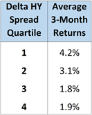
Source: Bloomberg, Verdad

These results indicate that three-month oil futures returns are highest when the three-month trailing change in the high-yield spread is low (i.e., in the first quartile). Conversely, three-month oil futures returns are lowest when the three-month trailing change in the high-yield spread is high (i.e., in the fourth quartile). We can further confirm this relationship by looking at a chart of the high-yield spread annotated with major oil price crashes over time.

Figure 4: High-Yield Spread (1954–2020) Annotated with Major Oil Price Crashes

Source: Bloomberg, Verdad

The chart shows that most major oil price crashes since the 1970s have coincided with the high-yield spread blowing out. This lends further credence to the idea that the high-yield spread, as a proxy for economic activity, can serve as a powerful indicator of the right—and wrong—times to be long oil.

We can turn this insight into a simple trading strategy: if, over the last three months, the high-yield spread has fallen, then our strategy goes long oil futures. We compare the performance of this strategy to a simple buy-and-hold strategy below.

Figure 5: Performance Indicators for Buy-and-Hold and HY Spread Strategies

Source: Bloomberg, Verdad

This strategy materially improves results relative to buying and holding: higher returns, lower volatility, reduced drawdowns, and a higher Sharpe ratio. However, the strategy is only invested 55% of the time, so the next challenge is to determine how best to allocate capital when not invested in oil futures. We consider three potential alternatives: the first strategy involves keeping the capital out of the market entirely when not invested in oil futures (“L/Out”); the second strategy goes long 10-year US Treasurys when not invested (“L/10YT”); and the third strategy adopts a shorting component based on the same high-yield signal, which ensures that the investor is either long or short oil futures at all times (“L/S”).

Figure 6: Performance Indicators for High-Yield Strategy with Different Combinations (1983–2020)

Source: Bloomberg, Verdad

The winning combination appears to be to go long oil futures when the high-yield spread is falling and to remain in 10-year US Treasurys when the high-yield spread is rising (the “L/10YT” strategy). This strategy generates the highest Sharpe ratio of the three options while also being successful in avoiding the colossal drawdowns that plague some of the other options like the fully exposed L/S model.

We can then see how this strategy would perform within the context of a traditional portfolio. Below, we compare the returns of a 60% stock, 40% bond portfolio to a portfolio comprised of 60% stocks and 40% this oil strategy.

Figure 7: Strategy in Context

Source: Bloomberg, Verdad

Combining this strategy with a traditional portfolio produces a strategy that outperforms both a traditional 60/40 and our oil strategy alone in terms of Sharpe ratio and drawdowns.

On a final note, although we used WTI futures to conduct all of our analyses, we could have also used Brent futures. Brent futures are newer and more thinly traded than WTI futures, but apart from that, the only salient difference is that Brent futures experience less severe drawdowns than WTI. As explained in this ICE article, this is largely because 1) Brent futures are cash-settled while WTI futures are settled with physical barrels and 2) WTI is a landlocked crude driven by regional fundamentals and storage constraints in Cushing, Oklahoma, while Brent is a seaborne crude driven by global fundamentals with far fewer storage constraints.

Conclusion

Investing in oil futures with a simple buy-and-hold strategy exposes investors to significant volatility and drawdowns without adequate compensation. But investors can reduce drawdowns and improve risk-adjusted returns by adopting a more nuanced strategy, one that uses the change in the high-yield spread as a guiding signal and a 60/40 approach that incorporates the S&P 500 into the portfolio.

Today, we note that the high-yield spread over the last three months has fallen materially (from 3.86 to 3.36), indicating that now could be a good time to implement our strategy on the long side. In the long run, we believe this strategy could produce excess returns and be a valuable diversifier to tailored investor portfolios.

Acknowledgment: This piece was co-authored by three of our term-time interns, David Balass, James Patton, and James Lockowandt. David previously studied finance and economics and is now finishing a double-degree in common and civil law (JD/BCL) at McGill University. James Patton is a freshman at Harvard currently pursuing a concentration in neuroscience with a secondary in economics. James Lockowandt is a sophomore at Harvard on an exchange year at the University of Oxford where he studies mathematics and philosophy. Both Patton and Lockowandt are actively seeking internship opportunities in finance for next summer, while Balass is seeking full-time employment at a value-focused hedge fund upon graduating law school in December.