Making the Most of Market Volatility
A practical approach to volatility modeling
Volatility forecasting isn’t just an academic exercise. Understanding and managing volatility is key to proper risk management for long-term portfolios.
The consequence of not paying attention is the pernicious and often overlooked phenomenon of volatility drag. Losses increase at the square of volatility: Go down 10% and up 10%, and you’ve lost 1%. Go down 20% and up 20%, and you’ve lost 4%. Go down 30% and up 30%, and you’ve lost 9%.
This math means that, all else equal, a smoother path leads to better outcomes. Forecasting volatility effectively, then, becomes more than a defensive tool. It can be a contributor to portfolio efficiency and performance.
Fortunately, it’s much easier to understand, model, and predict volatility than to predict returns. Returns are noisy, nonlinear, and prone to regime shifts. Volatility is much more predictable, with several characteristics that make a quantitative researcher’s task much easier:
Persistence: Volatility clusters. If markets were volatile yesterday, they’re likely to remain so today.
Mean Reversion: Elevated or suppressed volatility tends to revert toward more normal long-run levels.
Multi-Scale Structure: Volatility behaves differently across daily, weekly, and monthly horizons, reflecting the layered time frames of market participants.
Responsiveness to Shocks: Volatility doesn’t evolve in a vacuum. It reacts to macro announcements, earnings surprises, calendar effects, and signals from related markets.
Because this is such a tractable problem, the debate among practitioners isn’t whether volatility follows a random walk—we know it doesn’t—but rather which model works best. The most common approaches include:
Long-Run Average Volatility: A naïve but useful benchmark that assumes volatility reverts to a long-term mean.
Trailing Realized Volatility: Uses historical return variation over a fixed window. It’s simple, and surprisingly effective, especially in stable regimes.
EWMA (Exponentially Weighted Moving Average): Assigns greater weight to recent returns, allowing for quicker adaptation to shocks and regime changes.
GARCH (Generalized Autoregressive Conditional Heteroskedasticity): Models volatility as a function of squared return shocks and past conditional variances. Excels at short-term forecasting but is more complex to estimate and sensitive to structural breaks.
HAR (Heterogeneous Autoregressive) Model: Combines short-, medium-, and long-term realized volatility to capture how volatility propagates across time horizons.
We tested all of these models to identify the winner of the volatility prediction horserace.
Our favorite approach is the HAR model. Our research suggests that the HAR model, introduced by Corsi (2009), improves on earlier modeling approaches by best capturing the structure of volatility. Rather than relying on a single time period, HAR uses realized volatility measured from trailing daily, weekly, and monthly horizons, recognizing that traders and investors operate on different timeframes and that trailing volatility propagates forward at different rates. High-frequency traders respond to intraday movements, long/short funds may trade weekly or around event-driven setups, and allocators like pensions or sovereign wealth funds operate on slower monthly or quarterly cycles.
The standard HAR model follows the form:
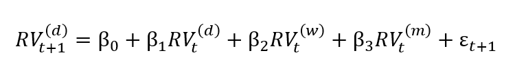
where RV denotes realized variance, typically estimated from squared daily returns (or higher-frequency return series).
HAR balances reactivity and stability by modeling future volatility as a weighted function of recent realized volatilities across multiple horizons. The coefficients are typically positive (capturing persistence) but sum to less than one, indicating mean reversion. Despite its simplicity, (a linear regression on lagged realized vol), HAR delivers strong out-of-sample performance.
Below, we compare the empirical performance of various models forecasting one-month forward volatility for several major asset classes: the Japanese Yen (JPY), Brent Oil Futures (OIL), the S&P 500 (SPX), and US Treasurys (UST).
Figure 1: Comparative Volatility Forecasting Performance (1M Horizon)
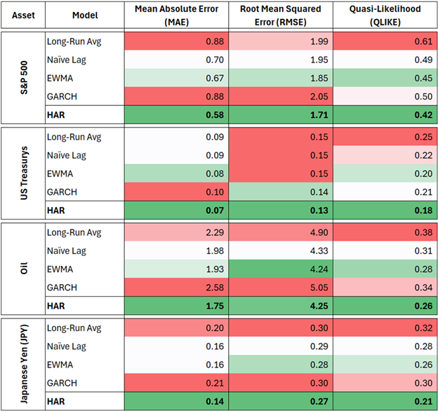
Source: Verdad analysis. Models evaluated against 30-day realized variance 1996-2025. Metrics shown are mean-absolute error (MAE), root-mean-square error (RMSE), and quasi-likelihood loss (QLIKE). Lower values indicate better fit. Forecasts are evaluated for five models—long-run average, naïve one-month RV lag, EWMA (λ = 0.94), GARCH(1,1) and HAR, applied to four assets (JPY, OIL, SPX, UST). Cells shaded green mark the best-performing model on each metric. QLIKE is chosen because it is robust to measurement noise and penalizes underestimated risk. Full model specifications appear in the linked technical appendix.
At a monthly horizon, HAR consistently outperforms alternative models across standard evaluation metrics such as MAE, RMSE, and QLIKE. This is consistent with prior research, which finds that HAR models are often more robust than more complex alternatives like GARCH when forecasting volatility beyond 10-day horizons.
While HAR provides a strong baseline for volatility forecasting, it relies solely on past realized returns and incorporates no forward-looking market information. One natural extension is to include a measure of market-implied volatility—such as the VIX (one-month forward implied volatility for the S&P 500)—to capture market participants’ expectations of future risk.
By adding VIX to the HAR model, we blend backward-looking realized volatility with a forward-looking signal distilled from options markets. Below we show how adding an implied volatility term improves over a baseline HAR model for the S&P 500.
Figure 2: HAR vs HAR-IV Forecast Evaluation (S&P 500)
Source: Verdad analysis. Models evaluated against 30-day realized variance of S&P 500 from 1996-2025. HAR model results are shown in green; HAR-IV results are shown in purple.
This enriched specification, sometimes referred to as HAR-IV, improves performance over the baseline model across all evaluation metrics. Outperformance tends to occur around sudden regime shifts or impending macro events, times when forward-looking options markets are pricing something that trailing realized volatility measures have not seen yet.
While many techniques exist for modeling volatility, we believe a lightweight HAR-IV model offers a practical, transparent, and effective solution for portfolio managers, particularly when managing risk over multi-day to multi-week horizons.