An Alternative Approach to Financial Modeling for Individual Companies
Nobel-prize winner Daniel Kahneman, his research partner Amos Tversky, and his student Philip Tetlock have revolutionized the science of forecasting. These scholars documented the limitations of our judgment and the best way to approach predicting the future.
The core of this new approach is “reference class forecasting.” The method is simple:
Identify a reference class
Obtain the statistics of the reference class
Use specific information about the individual case to adjust the baseline prediction relative to the reference class.
By establishing a base rate or outside view of the problem prior to analyzing the individual case, forecasters can significantly increase forecast accuracy.
Verdad applies these insights on forecasting to the world of investing. A few weeks ago, we looked at the statistics of the reference class of leveraged small value equities. This week, I wanted to talk more about the final step, of how to tailor the reference class forecast for an individual company.
The most important variables to model when analyzing an individual company are revenue growth, margin changes, and changes in exit multiple (See “Why most active managers fail”). We have studied a broad reference class of stocks to come up with base rates for each of these variables. We think investors should start with these “outside view” numbers in making forecasts and then adjust from there for individual companies. Here are the base rates we start with.
Revenue Growth
Revenue growth follows a random walk. Historical revenue growth has about a 25% correlation with future revenue growth and forecasting based on historical revenue trends is not an effective methodology, according to our research.
To demonstrate this insight, I took every company in the world that had a market capitalization of >$1 billion on 12/31/2004, 12/31/2007, and 12/31/2010. I then looked at 5-year revenue history and what happened over the following three years. As I mentioned, the correlation between the historical and future revenue growth was about 25%. Moreover, if you predicted that every company would grow 5% per year, that forecast would have been systematically more accurate than extrapolating from historical growth trends. We can see this graphically by dividing companies into quintiles of historical growth and tracking them into the future. In the below graph, year 5 is the sample date >Years 1–5 are the historical financials, while years 6–8 are the future.
Figure 1 Historical vs. Future Revenue Growth Rates by Quintile

Source: Verdad
As you can see, the lines become virtually indistinguishable relative to their historic rates at the time of sample. There’s still a slight correlation, with the higher growth quintiles outperforming the lower growth quintiles, but the spread between the quintiles is minimal.
The next question is the distribution of revenue growth: How volatile are these time series? The answer is extremely volatile. The standard deviation of revenue growth is about 150% of the mean, meaning if the mean growth is 10%, one standard deviation of revenue growth would range from -5% to 25%. If you’re trying to make a point forecast based on revenue growth, that wide standard deviation should be a clear reminder to be humbler and to broaden the range of expected potential outcomes.
Margins
Margins are, fortunately, a much easier time series to forecast. Companies’ margins tend to be fairly stable over time, and the standard deviation of margins is typically only about 10–20% of the mean. So if you’ve got a company with 10% margins, your range of outcomes should probably be 8–12% or so. Here’s a graphical representation of what dividing the world into margin quintiles looks like, with year 5 being the sample year.
Figure 2: Margins over Time
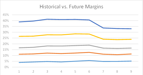
Source: Verdad
You can see some amount of margin compression across the board, with high margin companies typically suffering more. This is the result of competition in a capitalist world — typically, competitive advantages that drive high margins diminish over time. Assuming some level of margin compression is usually a safe bet for almost any company.
Multiples
Valuation multiples are a mean reverting time series. A safe assumption for companies above the median multiple is that their valuation multiples will cover 40% of the distance between their current level and the median over three years, while companies below median valuations typically cover 25% of the distance between their current level and the median over three years. See the table below of valuation multiples from 2001–2005 for the set of companies with market capitalizations >$1 billion in 2001.
Figure 3: EBITDA Multiples by Decile 2001–2005

Source: Verdad
Importantly, the correlation between historic and future multiples is reduced with time, and the standard deviation of multiples is about 30% of the historical mean.
Tying These Insights Together
We use Monte Carlo simulation models to generate probability distributions based on the above base rates. Given a set of probabilities for a set of different variables (revenues, margins, multiples), the Monte Carlo simulation will run hundreds or thousands of independent scenarios that reflect the probability distribution, and we can compare that probability distribution with the base rates of the broader reference class.
We start with the known knowns: the capital structure, historical financials, and market valuations of a given company. Followed by more mechanical variables like tax rate, interest rate, capital expenditure projections, etc. We then use the Monte Carlo model primarily to simulate changes in revenues, margins, and exit multiples, and to allow those different scenarios to play out through the financials.
I wanted to show how this looks for a few individual companies in our portfolio to give you a better understanding of the output this type of model would produce.*
Let me start with ARC Document Solutions (ARC). ARC sells software on recurring contracts to businesses, and it has historically had very stable revenue and margins, and almost no capital expenditure requirements. ARC has a fair amount of debt in the capital structure, and the company trades at a low multiple — historically ARC’s multiple has fluctuated significantly.
We made the following assumptions as guidelines for the simulation:
Mean annual revenue declines of 2% per annum, with a 3.4% standard deviation in line with the last five years of history
Mean EBITDA margins of 15.3% with standard deviation of 0.7% in line with the last five years of history
Mean EBITDA multiple of 7.0x with a 3.0x standard deviation in line with history, constrained such that if EBITDA declines the multiple must be lower than 6.0x (current EBITDA multiple) and if EBITDA grows it must be greater than 7.0x and is never lower than 3.5x or higher than 10x
All other cash flow and balance sheet items flowed mechanically from these assumptions
We forecast the following probability distribution for returns from investing in ARC:
Figure 4: Payout Distribution for ARC

ARC’s strong and stable cash flow generation ability provide a downside floor, while the company’s challenged market constrains the upside. ARC is stable, high-yielding investment that is unlikely to lose money, but it is also less likely to have the dramatic upside of other leveraged small value stocks.
In contrast, below I have modeled a Monte Carlo simulation for Kemet, a company that sells capacitators to the semiconductor industry. Kemet’s volumes and prices are very cyclical, and margins are dependent on raw material inputs that are also very volatile.
We modeled:
Volume growth of 2.5% with a standard deviation of 18%, in line with history
Prices varying with a 15% standard deviation relative to historical means
EBITDA exit multiple of 7.0x relative to 5.3x today, with a 6x standard deviation in line with the company’s history (with a minimum of 3x and a maximum of 15x)
With these assumptions, Kemet produces a very different distribution than ARC.
Figure 5: Payout Distribution for Kemet

The company has a high probability of bankruptcy, but it also has a higher probability of generating a >4x multiple of money over three years.
A leveraged small value portfolio comprises a mix of things that look like Kemet — though hopefully with uncorrelated end markets — and things that look like ARC. ARC’s returns are likely to be more dependent on free cash flow yield, while Kemet’s will be more dependent on industry volatility and multiple changes.
We believe these final steps in forecasting, adjusting the model relative to the reference class, is an important component of coming to the best and most accurate forecasts. Here we differ from purely quantitative investors who stop at the reference class and make no adjustments for individual securities.